Introduction

This is the second part of the work that attempts to find a recipe towards financial independence - a stage where you no longer need to work to support yourself.

In the previous article, we tried to formulate the problem of personal finance through a system of ordinary differential equations (ODE), which we later solved numerically using python. Given a set of input parameters, our numerical model was able to determine your financial condition (link).

In this article, we bring it to the next stage. We add randomness to the equation to account for life’s unpredictability. This time, we want to find out to what degree your financial success is really in your hands?

We will begin this journey by revisiting the math and add some random contributions. Then, we move into simulating some hypothetical scenarios using the so-called Monte Carlo method. Finally, we will use our augmented model to predict your chances with the help of the world’s historical data.

Let’s dive in.

Math revisited

The last model relied on a system two coupled differential equations, which we will reduce to just one for simplicity:

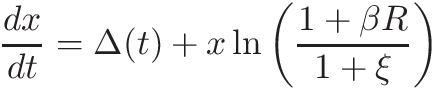
The equation models your total wealth by x, which is a time-dependent variable. Its left side is the derivative and the right side is composed of two contributing terms:

• Δ(t), which denotes a yearly balance: all income minus all expenses and taxes - simply how much is left after e.g. each year.
• xln(⋅), which denotes a combined force of investment and inflation that leads to compound interest. Note it’s proportionality to x itself, also more on why the terms reside under a logarithm you can find in the earlier article.

Here, the three parameters represent: B

• R - the expected average interest rate on your investment,
• ξ - the average yearly inflation rate,
• β ∈ [0,1] - a fraction of your wealth you choose to invest, which we’ll call the commitment factor.

Together, the second term can be represented with one number lnλ and understood as an effective interest rate. Consequently, whenever λ>1, you make money, and with λ<1 you lose.

The equation itself is a linear first-order differential equation, which can be solved analytically. However, since we will be “randomizing” it later, we will stick to the numerical methods and integrate it using python.

Important remark

We use normalized values for x and Δ to make the approach as generic as possible regarding any country, currency, or personal attitude. Therefore, Δ=1 can simply be interpreted as “you managed to save 100% of what you committed to”, which can, for example, translate to three months of a “financial pillow”.

This approach puts a person that earns 100k$ and spends 50k$ equally positioned to another that makes 10k$ and spends 5k$ in terms of financial independence. After all, financial independence is understood as a state under which x>0 and the amount that gets generated is positive despite Δ≤0. In other words, the growth at least compensates for the losses, and without a need for active work. Ergo, you can sit and eat forever.

Deterministic solutions

To find a solution, we need to calculate:

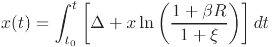
which to do numerically is just one function. Here, we arbitrarily set t0=25 and we model the balance function as

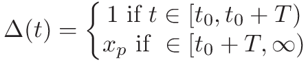
The first interval, we call an active time, as it represents the time, where most of us are actively employed and generating money. The second interval represents the retirement, with xp expressing balance during this time. To make things more difficult, we let xp<1. Thus, with a reasonable pension scheme, we can assume xp=0, meaning you can spend 100% of your pension and it won’t affect your total wealth.

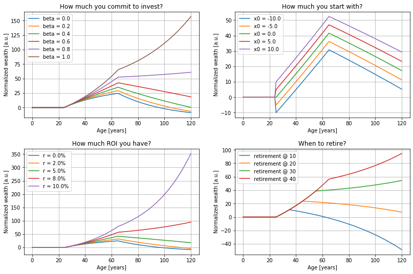
To test the influence of the different parameters, we show the progression of x under a different set of conditions (fig. 1). As we can see, high investment commitment β, high expected interest rates R, and longer active times T=t−t0 result in the solution to be found in the regime where growth generates more growth. Conversely, the initial condition x0=x(t0) does not affect growth at all - only the absolute amount of x.

Success condition

As mentioned earlier, our condition for financial independence is satisfied when x,dx/dt > 0 while Δ≤0. Another condition we should impose is that this stage is perpetual, meaning that once reached, there is no need to come back to a regular job.

However, once we have accounted for the randomness, the second condition would drive the point into a rather cumbersome analysis of the equation’s stability problem. To avoid that, and to account for a typical life scenario that is earning followed by spending, we will stick to representing the Δ as the following function

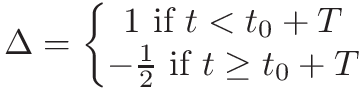
meaning that once you pass the retirement age, your yearly balance is expected to be -50% of your prior active time balance. We will, therefore, call it a success if once you get retired (t>t0+T), x stays positive, and the derivative of x gets positive on average.

Adding life’s randomness

This is an interesting part. The “master” equation offers us a solution for a perfectly deterministic world. Truth is that neither your condition nor (especially) the market’s are. Naturally, we need to account for some randomness in the process, but do it in a way such that our model still makes sense.

For this reason, we will replace the equation’s parameters with parametrized distributions. Then, we will use the so-called Monte Carlo method to find out where it leads us to. Once we collect the outcome through multiple iterations, we can use statistics to discuss the result.

Parametrization

The contributing factors can be divided into human-dependent and market-dependent. The human-dependent factors are Δ

and β as only these two can be influenced by your decisions. The contrary, R, and ξ are more of the world’s condition, which unless you are one of the Masonry, you have no influence on ;)

Mathematically, we can account for randomness to the balance function by injecting Gaussian noise in the following way:

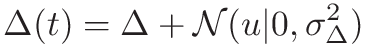
Where Δ is defined as earlier, and N is a zero-centered Gaussian noise of a specific variance.

Similarly, R and ξ can be modeled using a Gaussian noise as:

which can greatly “paint” human attitude towards investment in general.

Implementation

With this sort of weaponry, we can construct a “life-simulating” class.

class RealLife:
    def __init__(self):
        self.t0 = 25                        # starting age
        self.beta = np.random.beta(2, 5)    # somewhat natural
        self.mu_r = 0.05                    # investment rate avg
        self.sigma_r = 0.25                 # investment rate std
        self.mu_xi = 0.028                  # inflation avg  
        self.sigma_xi = 0.025               # inflation std
        self.x0 = 0.0                       # initial wealth
        self.balance_fn = self._rect        # balance fn (callable)
        self.sigma_delta = 2.0              # balance fn std
        
        self._rs = []
        self._xis = []
        self._deltas = []

    def live(self, x, t):
        delta = self.sigma_delta * np.random.randn()
        r = self.sigma_r * np.random.randn() + self.mu_r
        xi = self.sigma_xi * np.random.randn() + self.mu_xi
        
        self._rs.append(r)
        self._deltas.append(delta)
        self._xis.append(xi)
        
        rate = self.balance_fn(t - self.t0) \
             + np.log(1 + self.beta * r) * x \
             - np.log(1 + xi) * x
        return rate

    def _rect(self, t, t0, duration=30, floor=-0.5):
        x = np.where(t - t0 <= duration, 1.0, floor)
        mask = np.where(t > t0, 1.0, 0.0)
        return x * mask

Here, all parameters were set to resemble a real-life scenario, but the historical data based results are presented at the end.

It is also important to mention that self.beta is assumed to be time-independent. Consequently, we can interpret it as a situation that once a person is born (an object is instantiated), the investment commitment is chosen and stays the same. As we will use the Monte Carlo method, we should expect enough randomness across the population (after many runs).

Next, we need to integrate the new stochastic differential equation numerically. Since scipy.integrate.odeint performed poorly, we created our routine sdeint that matched the interface of odeint.

def sdeint(func, x0, t):
    x = np.zeros(t.size, dtype=float)
    x[0] = x0

    for i, dt in enumerate(t[1:]):
        x[i + 1] = x[i] + func(x[i], dt)

    return 

Finally, the simulation code can be wrapped in the following function.

import numpy as np
import pandas as pd

def simulate_with_random(you):
    t0 = np.linspace(0, you.t0 - 1, num=you.t0)
    t1 = np.linspace(you.t0, 120, num=(120 - you.t0 + 1))

    x_t0 = np.zeros(t0.size)
    x_t1 = sdeint(you.live, you.x0, t1)

    df0 = pd.DataFrame({'time': t0, 'x': x_t0})
    df1 = pd.DataFrame({'time': t1, 'x': x_t1})
    return pd.concat([df0, df1]).set_index('time')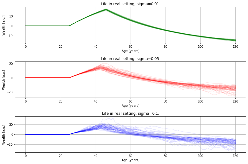

Monte Carlo

Now, we let it run for 1000 times, increasing the expected R. Besides, we randomize the active time T to fully randomize the population. Figure 3. shows the results.

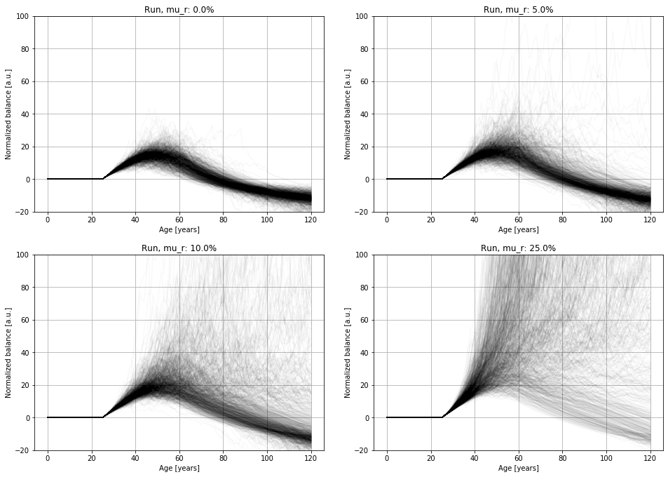
As we can see, whenever R<ξ it is virtually impossible to get into financial independence. This is because lnλ<0 and after integrating the solution experiences an exponential decay and the equation remains stable. However, increasing μR does not guarantee success either, due to the influence of the active time Tand the commitment factor β. Even for an artificially high μR, a large fraction of runs fails due to the reasons mentioned above.

Fortunately, both β and T are factors that depend on everyone’s personal choices. Therefore, if we freeze these to while letting R and ξ remain random, we should be able to estimate your chances of success at least to a certain extent.

Your chances against the historical data

To get a feeling for what it is like to combat the market, we need to  plug in some reasonable values of μR,σR,μξ and σξ. Assuming that “the history repeats itself”, we can argue that we can simulate the future using historical data. To get the values for inflation, we use the historical (1914-2020) data for the US from here. Similarly, to estimate the market’s behavior in terms of the mean and the variance, we use the S&P 500data from 1928-2020.

According to the data, we have ξ=3.24±4.98% and R=7.67±19.95%.

Next, we sweep T and β, while using the values we just computed.

from itertools import product


t = np.linspace(0, 120, num=121)
ACTIVE_TIME = np.linspace(10, 40, num=31)
BETAS = np.linspace(0.0, 1.0, num=11)
np.random.seed(42)

diags = []
for wy, beta in product(ACTIVE_TIME, BETAS):
    for _ in range(1000):
        you = RealLife()
        you.mu_r = 0.01 * mu_r          # S&P500 mean
        you.sigma_r = 0.01 * sigma_r    # S&P500 std
        you.mu_xi = 0.01 * mu_xi        # inflation mean
        you.sigma_xi = 0.01 * sigma_xi  # inflation std
        you.beta = beta                 
        you.balance_fn = lambda t: rect(t, you.x0, wy)
        df = simulate_with_random(you)

        passive = int(float(df[df.index > you.t0 + du] \
                    .diff().sum()) > 0)

        diags.append({
            'active': wy,
            'beta': you.beta,
            'avg_r': you.get_average_r(),
            'avg_delta': you.get_average_delta(),
            'avg_xi': you.get_average_xi(),
            'passive': passive,
        })

df = pd.DataFrame(diags)
df_agg = df[['active', 'beta', 'passive']] \
    .groupby(by=['active', 'beta'] \
    .mean() \
    .unstack() * 100

Final result

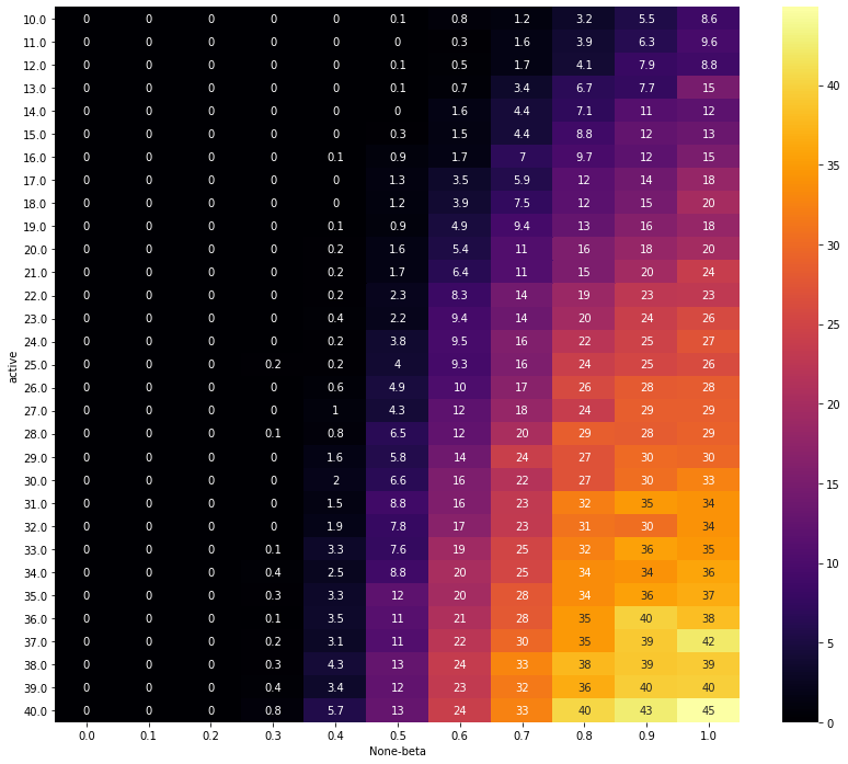
Figure 4. shows the final result of the Monte Carlo simulation for each (T,β)-pair. As we can see, any β<1/2 practically exclude you from ever becoming financially independent. Truth is that if you dream of securing a bright future for yourself, you need to learn to invest - whatever that means to you. This can mean anything from being a regular trader to a skilled entrepreneur - you need to learn to multiply what you have.

The second most important factor is your active time. This one, however, should be seen more as an “opportunity” window during which you can accumulate wealth. The longer it is, the higher the chances you will gain enough of the “fuel” to get your financial ship to fly.

However, even with 100% commitment and 40 years of hardship, the odds seem to play against you! Fortunately, you should remember that we used an oversimplified model for the Δ(t)

function. In reality, if you manage to translate what you learned into a higher salary and stay away from the temptation to overspend, your wealth will accumulate faster. Furthermore, nobody said you will be left to market “caprice”. Unless your only investment strategy is to safely allocate your money to some fund, you will probably learn to navigate and sail even during storms.

With that in mind, please find these results only as a way to encourage you to try, as they are not the ultimate recipe, but rather an attempt to figure out what matters. Good luck!

PS. If you want to play with the code and simulate for yourself, you can find the code on Github.