
In this article I would like to give you a brief introduction to Pandas, one of the most important toolkits Python provides for data cleaning and processing. I will show you some examples on how Pandas can be used to extract, explore and manipulate data.
You will learn how to read data into a DataFrame, how to query these structures, and how to write a DataFrame to a CSV file.
Why Python and Pandas?
At Webinterpret we are using Python and Pandas for Data Science tasks for a few reasons:
- Python is the fastest developing language for data science. With it's ever growing technological stack, it has some very strong data science libraries, including SciPy ecosystem and numerous packages for Machine Learning like XGboost or TensorFlow.
- Unlike R and other languages, Python is not just a statistical language, but also has full capabilities for data collection, cleaning, high performance computing and building production ready models that can be easily integrated with our applications.
The Pandas is an open source library created by Wes McKinney in 2008 and currently it is probably the most fundamental tool for almost every data scientist using Python. It provides a named vector and matrix-like structures, that help us see data in a tabular form, much like in Excel spreadsheets or in SQL databases. A concept of a DataFrame in Pandas is similar to a table in relational theory, so with some background in databases, you'll find Pandas fairly easy to work with.
Because it's open source and openly accessible, Pandas have very strong community, which drives the project forward and serves as an excellence point of reference. There are a couple of places you should consider visiting when looking for help with Pandas. Pandas documentation is a comprehensive source of information in the first place. However, often the best resource is simply Stack Overflow. It is used broadly within the Pandas community to post questions about this toolkit. Quiet often it happens, that questions tagged Pandas related are being answered by actual Pandas developer.
Ok. So now let's dig into Pandas.
Preparing environment
Before we start, we need to set up a virtual environment and install a few packages. For our convenience we will use Jupyter notebook, an open-source web based application that allows to work interactively with code and save the work in a form of notebooks.
$ mkdir pandas; cd pandas
$ virtualenv -p python3 env
$ source env/bin/activate
$ pip install pandas pandasql psycopg2 sqlalchemy jupyter pymongo tqdm
After all is installed you can check if jupyter notebook is working. Running below command should open a new tab in your browser:
$ jupyter notebook
As soon as jupyter is running and we've created a new notebook we can start writing code.
DataFrame Creation
First, we need to import pandas and numpy packages:
import numpy as np
import pandas as pd
Pandas toolkit introduces two very useful data structures: Series and DataFrame.
Series is a one-dimensional labeled array, capable of holding any data type (integers, strings, floating point numbers, Python objects, etc.). The axis labels are collectively referred to as the index.
DataFrame is a 2-dimensional labeled data structure with columns of potentially different types. You can think of it like a spreadsheet or SQL table, or a dict of Series objects. It is generally the most commonly used Pandas object.
This time we will be working mainly with DataFrames.
To create a DataFrame you can pass an array, and optionally name columns and indexes:
df = pd.DataFrame([[1,2,3], [4,5,6], [7,8,9]], columns=['A', 'B', 'C'], index=['a', 'b', 'c'])
df
| A | B | C | |
|---|---|---|---|
| a | 1 | 2 | 3 |
| b | 4 | 5 | 6 |
| c | 7 | 8 | 9 |
You can also create a DataFrame by passing a dict of objects that can be converted to series-like:
df2 = pd.DataFrame({'A' : 1.,
                    'B' : pd.Timestamp('20130102'),
                    'C' : pd.Series(1,index=list(range(4)),dtype='float32'),
                    'D' : np.array([3] * 4,dtype='int32'),
                    'E' : pd.Categorical(["test","train","test","train"]),
                    'F' : 'foo' })
df2
(excample from http://pandas.pydata.org/pandas-docs/stable/10min.html)
| A | B | C | D | E | F | |
|---|---|---|---|---|---|---|
| 0 | 1.0 | 2013-01-02 | 1.0 | 3 | test | foo |
| 1 | 1.0 | 2013-01-02 | 1.0 | 3 | train | foo |
| 2 | 1.0 | 2013-01-02 | 1.0 | 3 | test | foo |
| 3 | 1.0 | 2013-01-02 | 1.0 | 3 | train | foo |
Data Exploration
from pandasql import load_meat, load_births
#load example data
meat = load_meat()
births = load_births()

#return n top results, default is 5
births.head()
| date | births | |
|---|---|---|
| 0 | 1975-01-01 | 265775 |
| 1 | 1975-02-01 | 241045 |
| 2 | 1975-03-01 | 268849 |
| 3 | 1975-04-01 | 247455 |
| 4 | 1975-05-01 | 254545 |
To get insights into the data we can use two useful functions: info and describe.
births.info()
<class 'pandas.core.frame.DataFrame'>
RangeIndex: 408 entries, 0 to 407
Data columns (total 2 columns):
date      408 non-null datetime64[ns]
births    408 non-null int64
dtypes: datetime64[ns](1), int64(1)
memory usage: 6.5 KB
births.describe()
| births | |
|---|---|
| count | 408.000000 |
| mean | 320585.502451 |
| std | 29449.011996 |
| min | 236551.000000 |
| 25% | 303456.500000 |
| 50% | 325625.500000 |
| 75% | 342046.750000 |
| max | 387798.000000 |
And others:
births.columns
Index(['date', 'births', 'long_number'], dtype='object')
births.index
RangeIndex(start=0, stop=408, step=1)
births.head().values
array([[Timestamp('1975-01-01 00:00:00'), 265775],
       [Timestamp('1975-02-01 00:00:00'), 241045],
       [Timestamp('1975-03-01 00:00:00'), 268849],
       [Timestamp('1975-04-01 00:00:00'), 247455],
       [Timestamp('1975-05-01 00:00:00'), 254545]], dtype=object)
#transpose DF
births.head().T
| 0 | 1 | 2 | 3 | 4 | |
|---|---|---|---|---|---|
| date | 1975-01-01 00:00:00 | 1975-02-01 00:00:00 | 1975-03-01 00:00:00 | 1975-04-01 00:00:00 | 1975-05-01 00:00:00 |
| births | 265775 | 241045 | 268849 | 247455 | 254545 |
Sorting
#by an axis
births.sort_index(axis=0, ascending=False).head()
| date | births | |
|---|---|---|
| 407 | 2012-12-01 | 340995 |
| 406 | 2012-11-01 | 320195 |
| 405 | 2012-10-01 | 347625 |
| 404 | 2012-09-01 | 361922 |
| 403 | 2012-08-01 | 359554 |
# Sorting by values
births.sort_values(by='births', ascending=False).head()
| date | births | |
|---|---|---|
| 379 | 2008-08-01 | 387798 |
| 390 | 2011-07-01 | 375384 |
| 380 | 2008-09-01 | 374711 |
| 391 | 2011-08-01 | 373333 |
| 367 | 2007-08-01 | 369316 |
Working with indexes
# Set index
births = births.set_index('date')
births.head()
| births | |
|---|---|
| date | |
| 1975-01-01 | 265775 |
| 1975-02-01 | 241045 |
| 1975-03-01 | 268849 |
| 1975-04-01 | 247455 |
| 1975-05-01 | 254545 |
births = births.reset_index()
Selecting data
# Selecting columns
meat['beef'].head()
0    751.0
1    713.0
2    741.0
3    650.0
4    681.0
Name: beef, dtype: float64
meat[['date', 'beef', 'pork']].head()
| date | beef | pork | |
|---|---|---|---|
| 0 | 1944-01-01 | 751.0 | 1280.0 |
| 1 | 1944-02-01 | 713.0 | 1169.0 |
| 2 | 1944-03-01 | 741.0 | 1128.0 |
| 3 | 1944-04-01 | 650.0 | 978.0 |
| 4 | 1944-05-01 | 681.0 | 1029.0 |
# selecting by label
meat.loc[0:3, 'beef':'pork']
| beef | veal | pork | |
|---|---|---|---|
| 0 | 751.0 | 85.0 | 1280.0 |
| 1 | 713.0 | 77.0 | 1169.0 |
| 2 | 741.0 | 90.0 | 1128.0 |
| 3 | 650.0 | 89.0 | 978.0 |
# selecting by position
meat.iloc[1:6:2, [0,1,4]]
| date | beef | lamb_and_mutton | |
|---|---|---|---|
| 1 | 1944-02-01 | 713.0 | 72.0 |
| 3 | 1944-04-01 | 650.0 | 66.0 |
| 5 | 1944-06-01 | 658.0 | 79.0 |
# selecting by both label or position:
meat.ix[0:2, 'date':'pork']
| date | beef | veal | pork | |
|---|---|---|---|---|
| 0 | 1944-01-01 | 751.0 | 85.0 | 1280.0 |
| 1 | 1944-02-01 | 713.0 | 77.0 | 1169.0 |
| 2 | 1944-03-01 | 741.0 | 90.0 | 1128.0 |
meat.ix[0:2, 0:4]
| date | beef | veal | pork | |
|---|---|---|---|---|
| 0 | 1944-01-01 | 751.0 | 85.0 | 1280.0 |
| 1 | 1944-02-01 | 713.0 | 77.0 | 1169.0 |
| 2 | 1944-03-01 | 741.0 | 90.0 | 1128.0 |
#Filtering
meat[meat.date > '2000'].head()
| date | beef | veal | pork | lamb_and_mutton | broilers | other_chicken | turkey | cumulative | |
|---|---|---|---|---|---|---|---|---|---|
| 673 | 2000-02-01 | 2175.0 | 18.0 | 1558.0 | 20.0 | 2487.9 | NaN | 414.9 | 6673.8 |
| 674 | 2000-03-01 | 2300.0 | 20.0 | 1704.0 | 24.0 | 2687.9 | NaN | 469.7 | 7205.6 |
| 675 | 2000-04-01 | 2027.0 | 17.0 | 1398.0 | 23.0 | 2340.4 | NaN | 416.5 | 6221.9 |
| 676 | 2000-05-01 | 2303.0 | 19.0 | 1542.0 | 17.0 | 2741.7 | NaN | 492.3 | 7115.0 |
| 677 | 2000-06-01 | 2369.0 | 18.0 | 1538.0 | 17.0 | 2672.2 | NaN | 483.4 | 7097.6 |
Manipulating data
meat.sum(axis=1).head()
0    4410.0
1    4062.0
2    4068.0
3    3566.0
4    3788.0
dtype: float64
meat.mean()
beef               1683.463362
veal                 54.198549
pork               1211.683797
lamb_and_mutton      38.360701
broilers           1516.582520
other_chicken        43.033566
turkey              292.814646
cumulative         4384.466989
dtype: float64
meat.std()
beef                501.698480
veal                 39.062804
pork                371.311802
lamb_and_mutton      19.624340
broilers            963.012101
other_chicken         3.867141
turkey              162.482638
cumulative         1983.483767
dtype: float64
#creating a column
meat['foo'] = 'bar'
meat.head()
| date | beef | veal | pork | lamb_and_mutton | broilers | other_chicken | turkey | cumulative | examle | foo | |
|---|---|---|---|---|---|---|---|---|---|---|---|
| 0 | 1944-01-01 | 751.0 | 85.0 | 1280.0 | 89.0 | NaN | NaN | NaN | 2205.0 | foo | bar |
| 1 | 1944-02-01 | 713.0 | 77.0 | 1169.0 | 72.0 | NaN | NaN | NaN | 2031.0 | foo | bar |
| 2 | 1944-03-01 | 741.0 | 90.0 | 1128.0 | 75.0 | NaN | NaN | NaN | 2034.0 | foo | bar |
| 3 | 1944-04-01 | 650.0 | 89.0 | 978.0 | 66.0 | NaN | NaN | NaN | 1783.0 | foo | bar |
| 4 | 1944-05-01 | 681.0 | 106.0 | 1029.0 | 78.0 | NaN | NaN | NaN | 1894.0 | foo | bar |
meat['example'] = [np.random.random() for x in range(len(meat))]
meat.example.head()
0    0.317909
1    0.718370
2    0.026211
3    0.687999
4    0.290987
Name: example, dtype: float64
# Import garbage collector module
import gc
#
del meat['foo']
del meat['example']

# Collect garbage. It's expecially important to do it when working with large datasets and a little memory
gc.collect()
Use SQL syntax with pandasql
Pandasql (and also pysqldf) allows you to query pandas DataFrames using SQL syntax. It works similarly to sqldf in R. Pandasql seeks to provide a more familiar way of manipulating and cleaning data for people new to Python or pandas.
from pandasql import sqldf

#Specifying locals() or globals() can get tedious. You can defined a short helper function to fix this.
pysqldf = lambda q: sqldf(q, globals())

#Run a SQL query.It will insert given DF to SQLight DB in memory and then perform pd.from_sql() function.
#Warning: it is not the most efficient method and it often breaks on larger datasets
pysqldf("SELECT sum(beef), count(1) FROM meat;").head()
| sum(beef) | count(1) | |
|---|---|---|
| 0 | 1392224.2 | 827 |
More about Pandas vs SQL syntax: http://pandas.pydata.org/pandas-docs/stable/comparison_with_sql.html
Options and settings
births['long_number'] = 2234.0 * 2**100
births['long_number'].head()
0    2.831931e+33
1    2.831931e+33
2    2.831931e+33
3    2.831931e+33
4    2.831931e+33
Name: long_number, dtype: float64
#suppress displaying long numbers in scientific notation
pd.set_option('display.float_format', lambda x: '%.2f' % x)
births['long_number'].head()
0   2831931440909864482943634960809984.00
1   2831931440909864482943634960809984.00
2   2831931440909864482943634960809984.00
3   2831931440909864482943634960809984.00
4   2831931440909864482943634960809984.00
Name: long_number, dtype: float64
#reset option
pd.reset_option('display.float_format')
More about options and settings at:
http://pandas.pydata.org/pandas-docs/stable/options.html
Getting Data In/Out
#CSV
meteorites = pd.read_csv('Meteorite_Landings.csv')
meteorites.head()
| name | id | nametype | recclass | mass (g) | fall | year | reclat | reclong | GeoLocation | |
|---|---|---|---|---|---|---|---|---|---|---|
| 0 | Aachen | 1 | Valid | L5 | 21.0 | Fell | 01/01/1880 12:00:00 AM | 50.77500 | 6.08333 | (50.775000, 6.083330) |
| 1 | Aarhus | 2 | Valid | H6 | 720.0 | Fell | 01/01/1951 12:00:00 AM | 56.18333 | 10.23333 | (56.183330, 10.233330) |
| 2 | Abee | 6 | Valid | EH4 | 107000.0 | Fell | 01/01/1952 12:00:00 AM | 54.21667 | -113.00000 | (54.216670, -113.000000) |
| 3 | Acapulco | 10 | Valid | Acapulcoite | 1914.0 | Fell | 01/01/1976 12:00:00 AM | 16.88333 | -99.90000 | (16.883330, -99.900000) |
| 4 | Achiras | 370 | Valid | L6 | 780.0 | Fell | 01/01/1902 12:00:00 AM | -33.16667 | -64.95000 | (-33.166670, -64.950000) |
#SQL
from sqlalchemy import create_engine
localhost = 'postgresql://user:pass@localhost:port/db'
engine = create_engine(localhost)

df = pd.read_sql("select * from tablename limit 100", engine)
#JSON
df = pd.read_json('JEOPARDY_QUESTIONS1.json')
df.head()
# Write out data to CSV
df.to_csv('jeopardy.csv')
Reading MongoDB \ JSON normalization
# read from MongoDB
from pymongo import MongoClient
uri = 'mongodb://user:pass@url/db'
client = MongoClient(uri)
db = client['db_name']
cursor = db.collection.find().limit(100)
df = pd.DataFrame(list(cursor))
#JSON normalization when dealing with nested documents

from pandas.io.json import json_normalize

cursor = db.collection.find()
df = json_normalize(list(cursor))
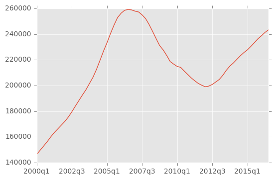
Visualization Example
#  for simple graphic embedded in the notebook use
%matplotlib inline

# for more interactive plot use
# %matplotlib notebok

import matplotlib
import matplotlib.pyplot as plt
def convert_data_to_quarters():
    '''
    Converts the housing data to quarters
    and returns it as mean values in a dataframe.
    '''
    #read data from  csv
    df = pd.read_csv('City_Zhvi_AllHomes.csv')
    # create a multi index of State and RegionName
    df = df.set_index(["State","RegionName"])
    # select only interesting columns
    df = df.iloc[:,49:]
    # convert column names to datetime
    df.columns = pd.to_datetime(df.columns)
    df = df.resample('Q',axis=1).mean()
    df.columns = list(map(lambda x: '{}q{}'.format(x.year, x.quarter), df.columns))

    return df

df = convert_data_to_quarters()
# Change style of a plot
matplotlib.style.use('ggplot')

df.describe().transpose()['mean'].plot()
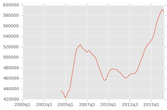
ny = df.iloc[0]
ny.plot()
Links
10 minutes to Pandas:
http://pandas.pydata.org/pandas-docs/stable/10min.html
Pandas vs SQL: syntax comparison:
http://pandas.pydata.org/pandas-docs/stable/comparison_with_sql.html

