
Background
At the time of writing Webinterpret is managing over one hundred million online product listings. To maximize our efficiency we need to know which are worth localizing into foreign markets. It is very valuable to know which have the best chance to sell and increase the our customer's revenue without unnecessarily increasing their listing fees.
A long time ago we employed a very simple formula to evaluate the quality of our listings. We scored them based on their price and past sales (forthwith referred to as GMV):
$$ listing~score = 2 \cdot \sum_i^N{domestic~sales_i} + 1 \cdot \sum_i^M{international~sales_i} + 0.5 \cdot item~price $$
[equation 1]: old scoring formula
The higher the score (forthwith referred to as salesrank), the higher the chance an item would be chosen to list internationally.
It is not hard to see there may be some problems with this approach:
- some items are country-specific and sell only in the domestic market (domestic transactions don't matter here)
- vastly overpriced items without any competitive advantages don't have any greater chance to sell
- there are items that sell well only during specific times of the year (snowboards sell better in winter, bicycles sell better in summer)
These and other issues suggest that the salesrank needed to be calculated more carefully.
Investigation of the simple scoring formula
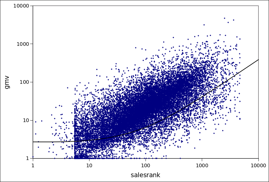
Do localized items with higher salesrank really generate more revenue?
To check this question we visualize the correlation of the calculated simple salesrank with the GMV of the corresponding localized (Y axis) as a scater plot. This shows a low positive correlation between the salesrank and GMV i.e. that GMV of items with higher salesrank may be on average a bit higher than those with lower salesrank.
Another interesting observation is that we can also use our calculated salesrank to roughly estimate the sales, even on small batches of product listings. The error will be very high for now but we are going to do better!
An improved formula for scoring product listings
At Webinterpret we have acquired a lot of domain knowledge about rating and optimizing online product listings. We know which items are more likely to sell well and we can use this knowledge in our scoring formula.
New formula
The formula for our improved salesrank is a generalized equation [1]:
$$ S_{new} = F(s_i) = F(s_1, s_2, ..., s_N) $$
[Equation 2]: generalized scoring formula
where \(s_i\) is a numerical representation of a single feature.
A simple example would be:
$$ S_{new} = \sum_i^N{ c_i \cdot s_i}$$
[Equation 3]: a simple implementation of equation [2] - linear combination of features
or more generally:
$$ S_{new} = \sum_i^N{ \sum_{k=0}^M{ c_{(i,k)} \cdot s_i^k}} $$
[Equation 4]: a more precise implementation of equation [2]
where \(s_i\) is a salesrank component derived from a part of our knowledge and \(c_i\) is a weight associated with this part of knowledge. \(c_i\) should be proportional to the positive impact of a feature on the item. Similarly, negative values indicate that a feature makes certain items less likely to sell.
M is the max degree of polynomial we want to fit. For \(M \rightarrow \infty\) this polynomial will represent an analytic function while a lower degree polynomial will be an approximation of this function (see Taylor series).
We may also assume that the features are not independent and therefore \(F(s_i)\) may have a much more complicated form.
Knowledge components
Equation [2] enables us to define more and more components to improve the accuracy of our recommendation.
Such components include:
- item price (more expensive items may be worth listing first)
- item transactions (items sold in their domestic market have bigger chance to sell well after localizing them properly)
- number of listing views (the more people see a listing, the more can buy it)
- free shipping/multiple shipping options available (people tend to prefer listings with such options enabled)
- item condition (people are more likely to buy new items, than used ones, or these with defects)
- item category (people are more likely to buy electronics than books)
- features which promote items in the search engine of it's shopping portal (it will be higher in search results so it is more probable to be bought)
This list can be extended easily and may also include collective data:
- seasonality (to utilize people's buying patterns)
- keywords analysis in listing title (to improve searchability of our listings)
- description analysis (to promote listings with more appealing descriptions)
We can also incorporate some external forecasts of buying demand or trends to boost the results.
Finding the coefficients for the recommendation formula
Using our archive of items and the historical GMV generated from the asociated localized items we are trying to find weights associated with every feature such that correlation:
$$ corr(G, S) = max $$
In general, formula [2] may be found using genetic programming or other optimization techniques. We are looking for pairs:
$${G, F(s_1, s_2, ... , s_N)}$$
such that
$$corr(G, F(s_1, s_2, ... s_N)) = max $$
where G is GMV (fixed) and \(F(s_1, s_2, ... s_N)\) is the new salesrank using an extended set of features and weights.
Approaches to find a better recommendation formula
Multiple approaches could be taken to solve the equation [4].
One can apply deterministic or evolutionary methods to find weights \(c_{(i,k)}\). Methods such as: gradient descent, genetic algorithms or simulated annealing come in handy.
One can also find the whole non-linear function F from equation [2] using genetic programming techniques.
A different approach could also be taken -- one could train a neural net to predict GMV based on item features.
Visualization of the results
Different sets of item features can be used in optimizing the formula.
Now let's go through some simple examples that are easy to visualize:
2 features (2 dimensions)
We are looking for weights for a simple formula:
$$S = c_1 \cdot gmv~domestic + c_2 \cdot gmv~international $$
The feature space looks like this:
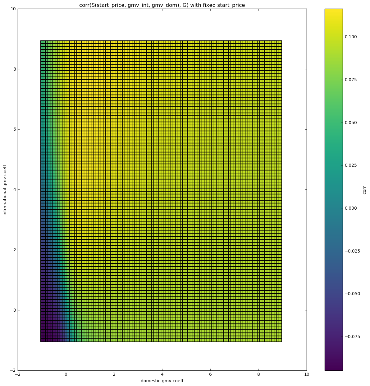
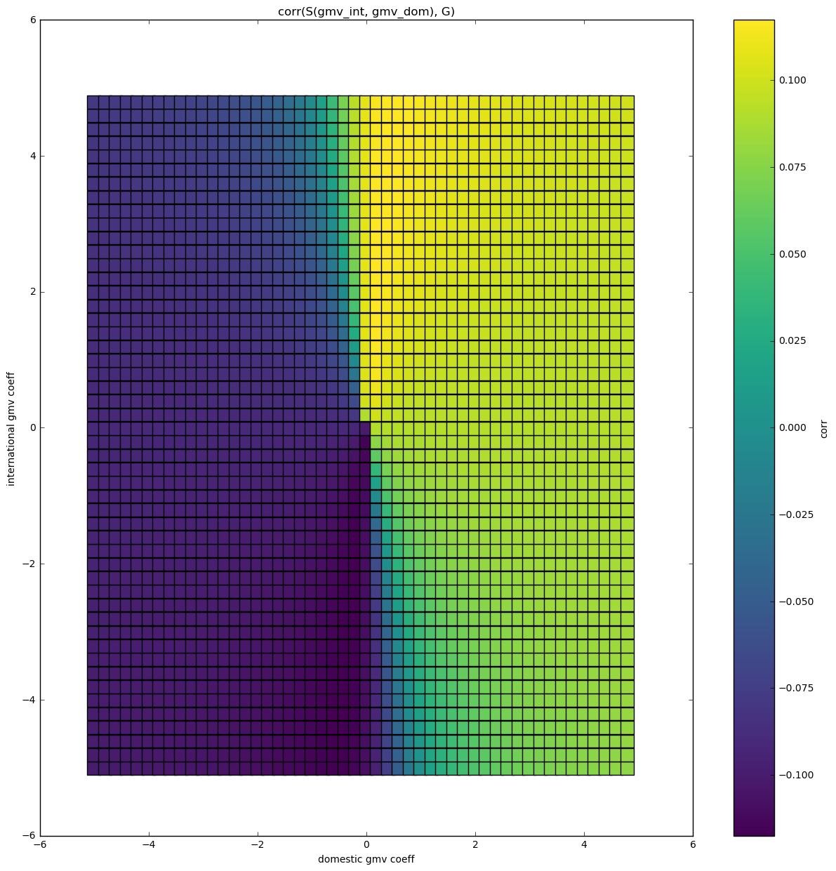 Correlation space - 2 features
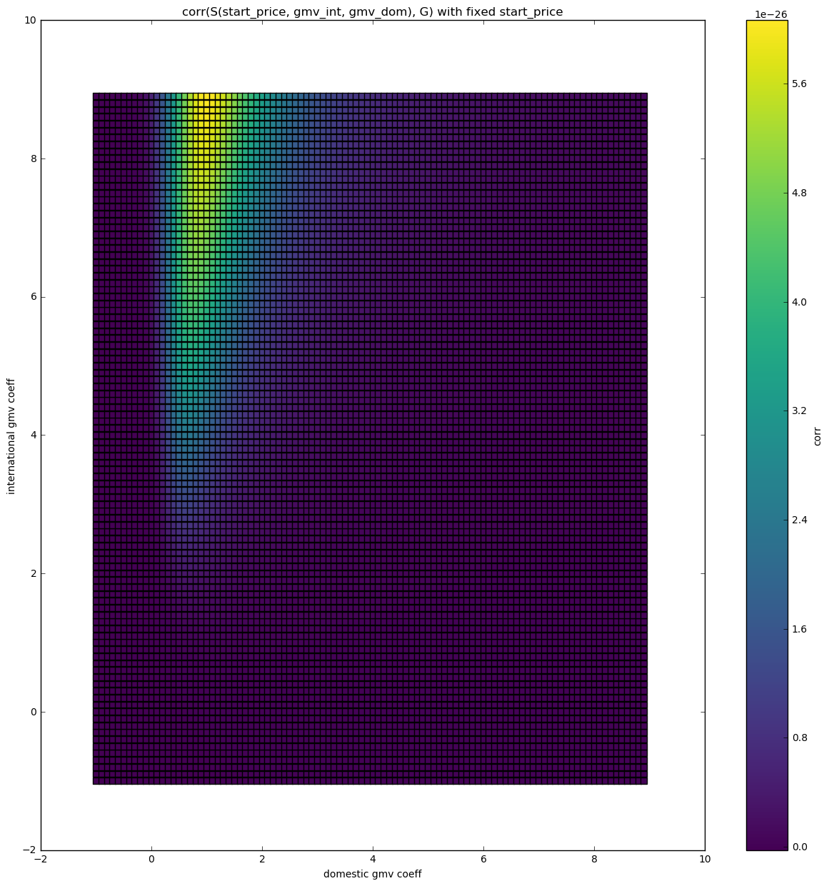
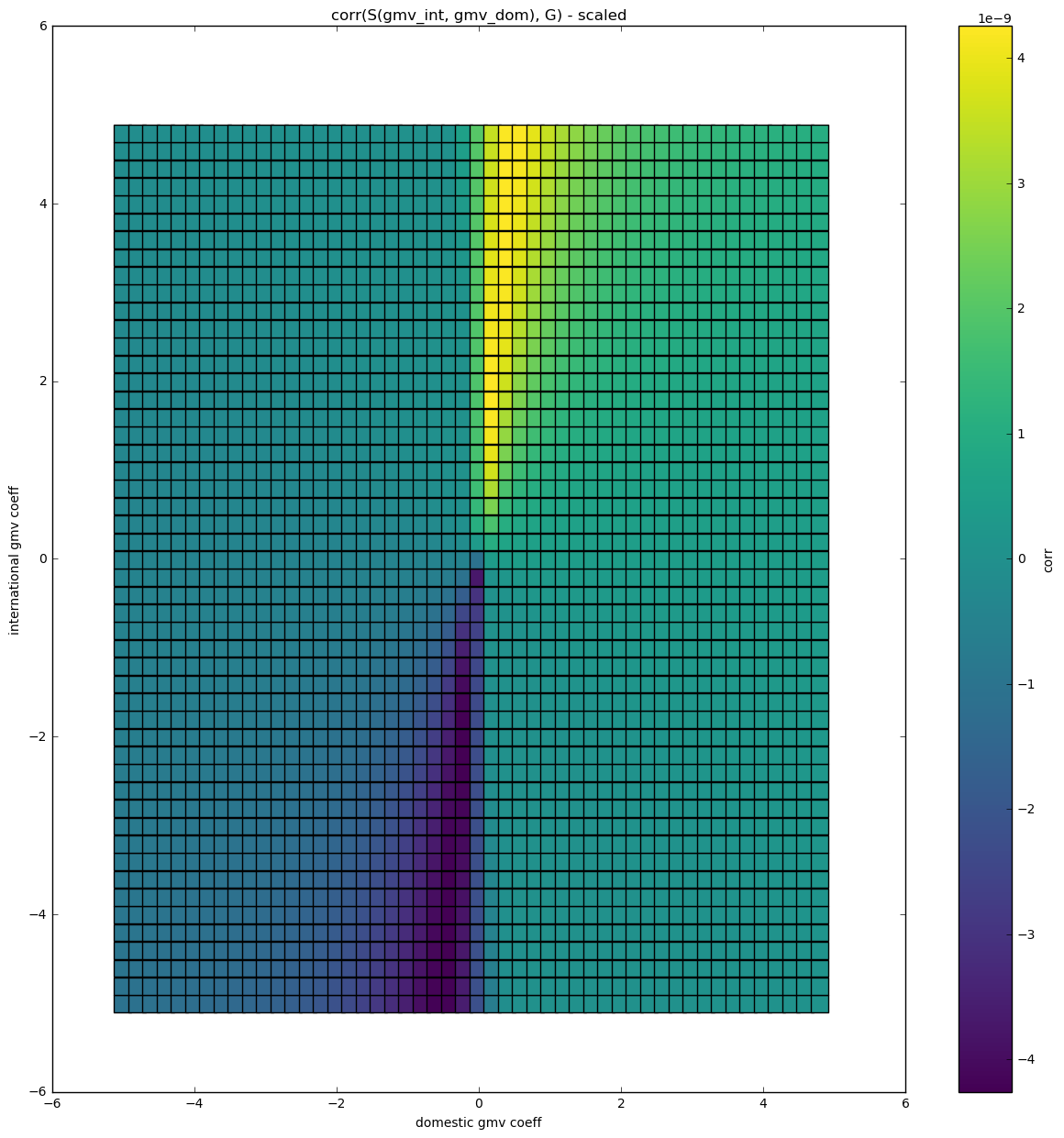 Correlation space - 2 features - difference amplified
On the second image the difference was amplified to improve the visual experience.
We can see that there are regions with either positive or negative correlation. So different weights associated with different features indeed bring different results. Let's explore this further.
Dimensionality reduction
One helpful property of correlation is that
$$corr(cX, Y) = corr(X, Y)$$
This enables us to make one of the weights fixed and just fit the other one. Let's take the previous formula and fix the coefficient of $gmv_domestic$.
$$ S' = gmv~domestic + \frac{c_2}{c_1} \cdot gmv~international = gmv~domestic + c_1' \cdot gmv~international$$
We can interpret this as taking a slice through the previous chart. Fortunately it contains all information that is relevant to us.
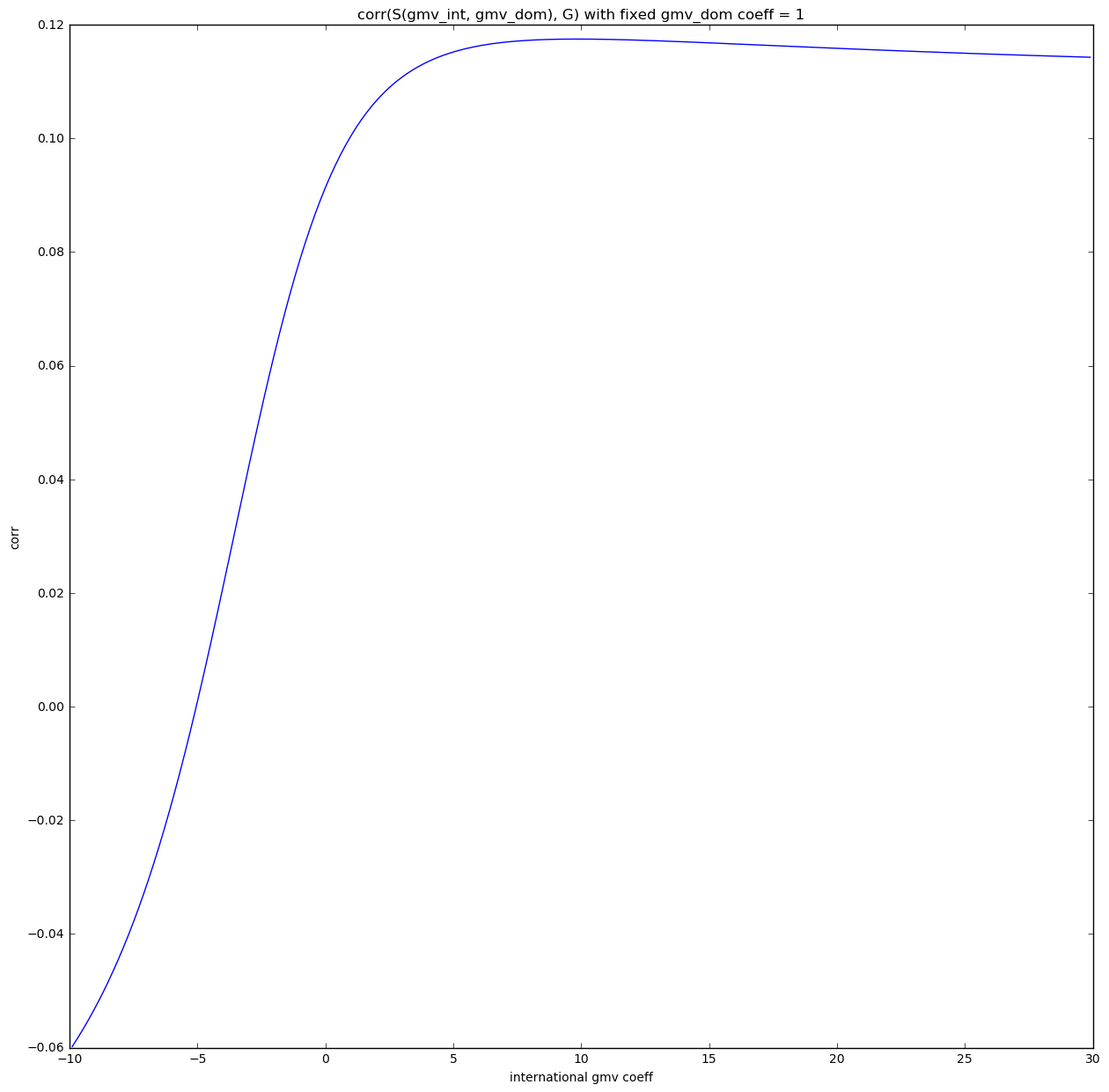 Correlation space - 2 features
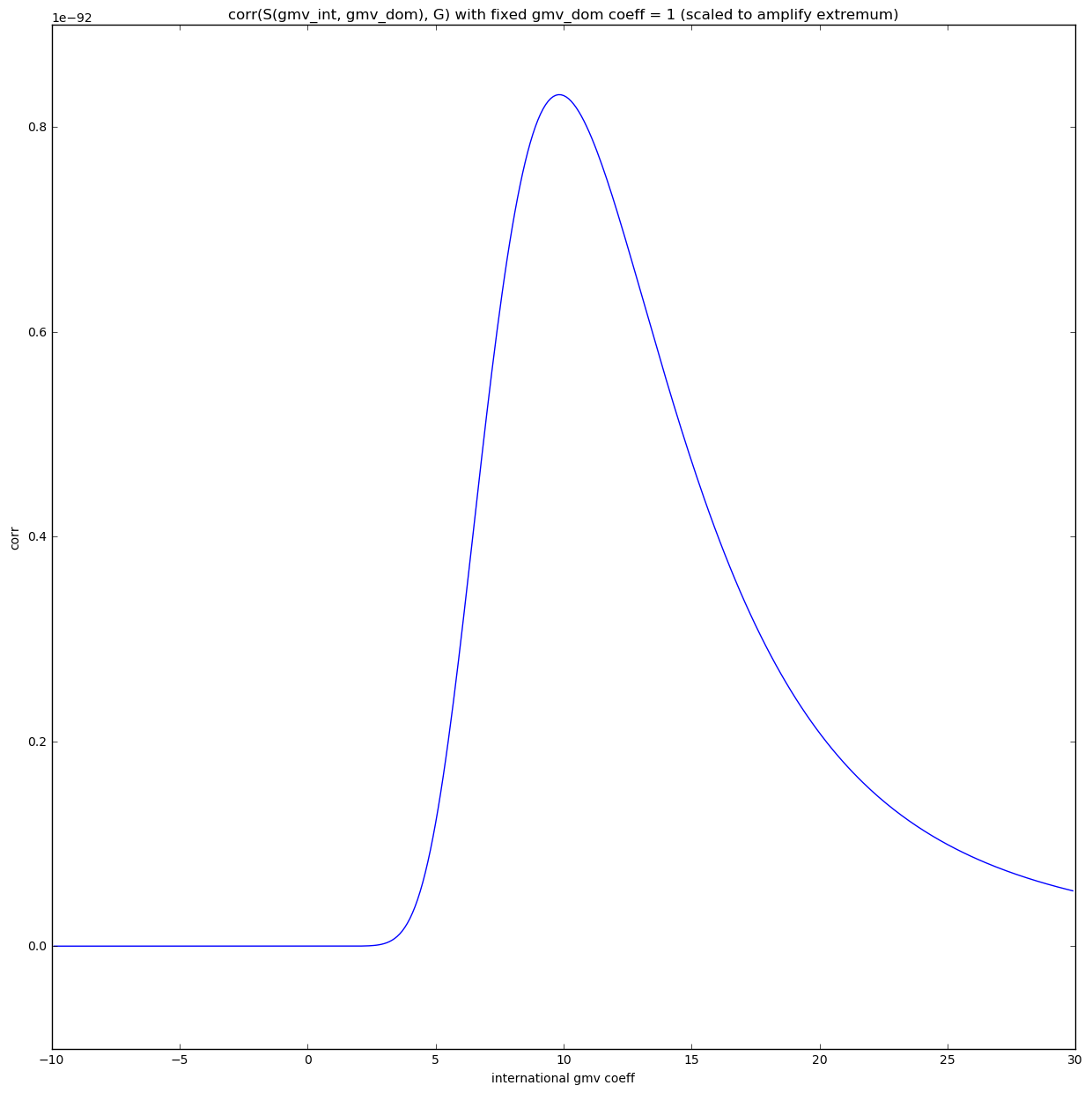 Correlation space - 2 features - difference amplified
Now we can clearly see that the function \(F = corr(G, S({gmv~int}, {gmv~dom}))\) is smooth with no multiple local maxima so we can find the solution using methods based on gradient descent. This should be fine as long as we are considering only linear combinations of features.
For this particular set of features we can see that correlation reaches it's max at \( gmv~dom = 1\), \(gmv\_int \approx 10\)
3 features (reduced to 2 dimensions)
Now let's add another feature -- item price.
$$S = start~price + c_1 \cdot gmv~domestic + c_2 \cdot gmv~international$$
Start price is fixed, domestic gmv and international gmv are variable.
 Correlation space - 3 features - difference amplified
 Correlation space - 3 features - difference amplified
Here we can see that when the start price coefficient is set to 1, international and domestic sales coefficients should be positive and the international sales coefficient should be greater than the domestic sales coefficient.
4 features (reduced to 3 dimensions)
Let's add one more feature -- the number of listing views.
The equation we are trying to optimize now looks like this:
$$ corr(G, S) = max$$
where
$$ S = start~price + c_1 \cdot gmv~domestic + c_2 \cdot gmv~international + c_3 \cdot listing~views $$
At this point an exhaustive search of the solution space would already take too much time (over 24 hours for the previous sample). This time specialized solvers will be used to find a solution without checking the whole space within a given boundary.
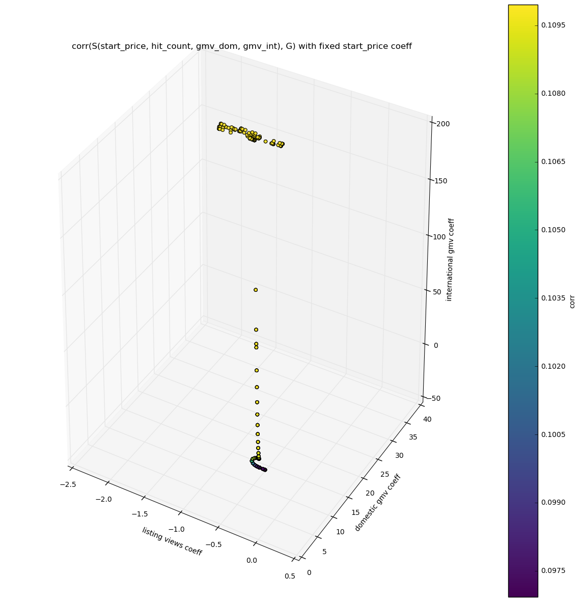 Several steps in correlation space - 4 features
Looking at the chart above we can see that the best set of coefficients found for the chosen features are:
- 1 for item price (fixed)
- approx 15 for domestic sales
- approx 200 for international sales
- approx -0.5 for listing views
This shows again that international GMV is the most important predictor of sales on localized items. Domestic sales are also quite important. The price of the item does not matter that much. The number of listing views is very weakly negatively correlated with sales on the localized items.
More features
As we can see, adding more features brings us more and more insight into sellers behaviour. However, because spaces of higher dimensionality are hard to bisualize we will leave them to your imagination. There may be a more detailed post on this one day in the future.
Results
Experimenting with different sets of features and different order of polynomials in equation [2] enabled us to find a combination of features that boosted the correlation between our calculated salesrank and GMV from 0.144 to 0.248.
In this specific example 5 features were chosen and the highest order of each feature in the polynomial was 2. We had to find 10 coefficients for our scoring equation. This was a trade-off between effectiveness (the effect should be clearly visible) and computing time (it shouldn't take more than several hours for a data sample which contains a few million items).
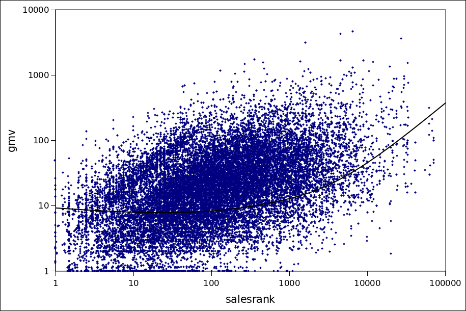 GMV(salesrank) - before optimization
 GMV(salesrank) - after optimization
Indeed, the charts show that the salesrank of items calculated with the new formula is more strongly correlated with their GMV.
Conclusion
In this short article I presented a basic framework to explore and improve online listing scoring.
I showed some simple techniques which, given enough data, can be applied to promote better listings, understand customers' behaviour and estimate profit that can be gained from online product listings.
The presented model can be greatly improved, mostly by using a bigger set of meaningful features and is a constant work in progress.

